library("jsonlite")
library("tidyverse")
library("xml2")
library("RCurl")
library("scales")
library("purrrlyr")
plays <- fromJSON("data/music-data-2018.json")If your social media feed is anything like mine, you probably see a lot of posts like this toward the end of the year.
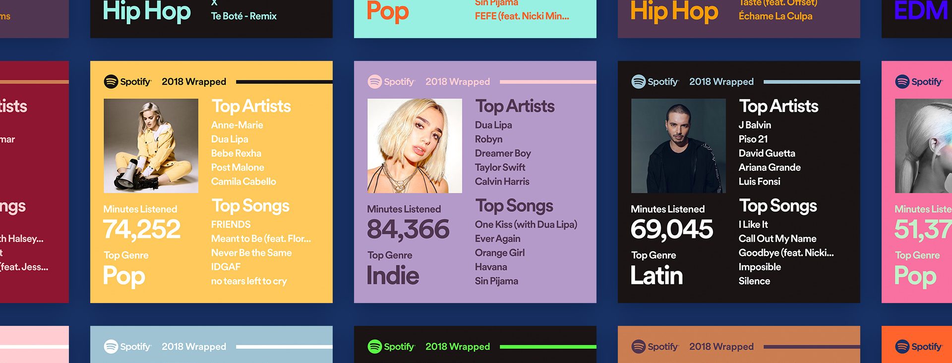
It can be fun to see what kind of music other people like and to share your own music tastes. It’s also a great advertisement campaign for Spotify (see their nice logo in the top left of these graphics).
The only problem for me is that I’m not a Spotify user, so when I try to open my #2018Wrapped data, I am greeted with a very nicely packaged empty box. Fortunately, as I wrote about in my last post, I log all of my music streaming using a free, open-source service called ListenBrainz. I am going to use that data to create my own end-of-year music graphic similar to the ones posted by my friends who use Spotify.
The Data
I’m doing this project in R for a couple of reasons. First of all, I kind of like R. Honestly this wasn’t the case a few years ago. It has tons of great stats tools, but a lot of things are very much designed for statisticians.
I’m only interested in my activity from 2018, so I will filter my dataset down to only the entries with a timecode in 2018.
stamp <- as.numeric(as.POSIXct("2018-01-01", format = "%Y-%m-%d"))
recentPlays <- plays[plays$timestamp >= stamp, ]
recentPlays <- as_tibble(recentPlays[
c("artist_name", "track_name", "release_name", "timestamp")
])
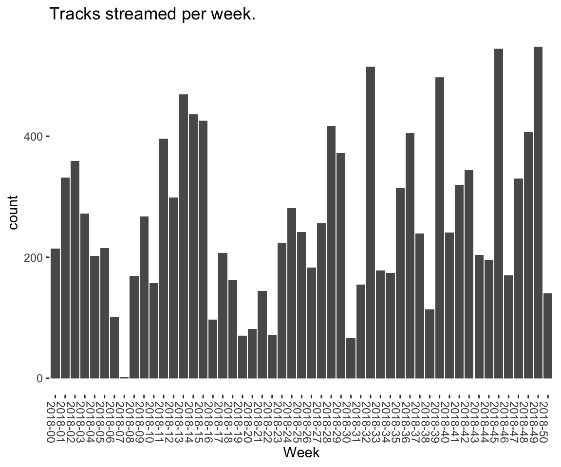
nrow(recentPlays)[1] 13226That’s a lot of music! How was that listening distributed over time?
recentPlays$date <- as.POSIXct(recentPlays$timestamp, origin = "1970-01-01") %>%
    as.Date()
recentPlays %>%
    ggplot(., aes(format(date, "%Y-%U"))) +
    geom_bar(stat = "count") +
    labs(x = "Week", title = "Tracks streamed per week.") +
    theme(
        axis.text.x = element_text(angle = -90, hjust = 0),
        panel.border = element_blank(),
        legend.key = element_blank(),
        panel.background = element_blank(),
        plot.background = element_rect(fill = "transparent", colour = NA)
    )
Top Artists
We can use this data to answer some pretty easy questions. For example, who were my top artists in 2018?
| artist_name | n |
|---|---|
| Charli XCX | 870 |
| Carly Rae Jepsen | 427 |
| Ariana Grande | 311 |
| Kacey Musgraves | 277 |
| Marina And The Diamonds | 223 |
| Lady Gaga | 215 |
Top Songs
I can also do something similar to find my top tracks for the year.
| artist_name | track_name | n |
|---|---|---|
| SOPHIE | Immaterial | 41 |
| Charli XCX | No Angel | 40 |
| Charli XCX | I Got It (feat. Brooke Candy, CupcakKe and Pabllo Vittar) | 36 |
| Charli XCX | Focus | 34 |
| Charli XCX | Lucky | 33 |
I listen to a lot of Charli XCX, so this list doesn’t really have a lot of variety (though Charli is absolutely one of the most versatile artists in pop today). Let’s filter the results to only show one song per artist.
top_songs <- recentPlays %>%
    group_by(artist_name, track_name) %>%
    count(sort = T) %>%
    ungroup() %>%
    distinct(artist_name, .keep_all = T) %>%
    head(5)
top_songs| artist_name | track_name | n |
|---|---|---|
| SOPHIE | Immaterial | 41 |
| Charli XCX | No Angel | 40 |
| Troye Sivan | My My My! | 32 |
| Kacey Musgraves | High Horse | 31 |
| Carly Rae Jepsen | Party For One | 26 |
Top Albums
ListenBrainz also logs the release name, so it’s pretty easy to compile a list of my top albums.
topAlbums <- recentPlays %>%
    group_by(artist_name, release_name) %>%
    count(sort = T)
topAlbums %>% head()| artist_name | release_name | n |
|---|---|---|
| Charli XCX | Pop 2 | 296 |
| Kacey Musgraves | Golden Hour | 247 |
| Carly Rae Jepsen | Emotion (Deluxe) | 191 |
| Marina And The Diamonds | Electra Heart | 179 |
| Charli XCX | Number 1 Angel | 153 |
| Ariana Grande | Dangerous Woman | 144 |
Let’s say I just want to know which albums from the last year I streamed.
getAlbum <- function(row) {
    mburl <- sprintf(
        'https://beta.musicbrainz.org/ws/2/release/?query=artist:%s+release:%s+AND+status:official+AND+format:"Digital%%20Media"&inc=release-group&limit=1',
        curlEscape(row$artist_name),
        curlEscape(row$release_name)
    )
    Sys.sleep(0.25)
    groupData <- read_xml(mburl)
    xml_ns_strip(groupData)
    release <- xml_find_first(groupData, "//release[@ns2:score=100]")
    xml_ns_strip(release)
    # If it is empty
    if (class(release) == "xml_missing") {
        release <- xml_new_document() %>% xml_add_child("")
    }
    # Go with the earliest release date given.
    date <- xml_text(xml_find_first(release, "//date"))
    artistId <- xml_text(xml_find_first(release, "//artist/@id"))
    df <- data.frame(date, artistId, stringsAsFactors = FALSE)
    colnames(df) <- c("date", "artistId")
    return(df)
}
recentAlbums <- topAlbums %>%
filter(n > 100) %>%
by_row(..f = getAlbum, .to = ".out") %>%
unnest(cols = c(.out))
recentAlbums %>%
filter(str_detect(date, "2018")) %>%
dplyr::select(artist_name, release_name, n, date) %>%
filter(n > 75)| artist_name | release_name | n | date |
|---|---|---|---|
| Kacey Musgraves | Golden Hour | 247 | 2018-03-30 |
| Clarence Clarity | THINK: PEACE | 119 | 2018-10-04 |
| SOPHIE | OIL OF EVERY PEARL’S UN-INSIDES | 119 | 2018-06-15 |
| Amnesia Scanner | Another Life | 118 | 2018-09-07 |
| Troye Sivan | Bloom | 118 | 2018-08-31 |
| IDLES | Joy as an Act of Resistance. | 103 | 2018-08-31 |
Minutes streamed
Initially I considered a brute-force approach to this problem; however, it does not seem a good use of resources to get the length for every single song. Instead I’ll write a function to grab lengths for songs…
getLengths <- function(row) {
    song_stripped <- trimws(sub("\\(.*\\)", "", row$track_name))
    mburl <- sprintf(
        "https://beta.musicbrainz.org/ws/2/recording/?query=artist:%s+AND+recording:%s&limit=2",
        curlEscape(row$artist_name),
        curlEscape(song_stripped)
    )
    # To comply with the rate limit.
    Sys.sleep(0.5)
    albumData <- read_xml(mburl)
    xml_ns_strip(albumData)
    length <- xml_integer(xml_find_first(albumData, "//length"))
    return(length)
}
…and sample 100 of my streams.
This gives me a reasonable mean length.
Which I can use to estimate the total for the population.
mins <- nrow(recentPlays) * mean(as.numeric(mean_len)) / 60000
mins
[1] 50858.81Top Genre
Observation: the top quartile of artists make up the vast majority of my streams this year.
top_artist_ids <- recentAlbums %>%
    group_by(artistId) %>%
    filter(!is.na(artistId)) %>%
    summarize(Sum = sum(n)) %>%
    arrange(desc(Sum))
top_artist_ids %>%
summarize(sum(Sum))| sum(Sum) |
|---|
| 2294 |
Conclusion: This is a good time to use a sample again.
fetchGenres <- function(row) {
    mburl <- sprintf(
        "https://beta.musicbrainz.org/ws/2/artist/%s?inc=genres",
        row$artistId
    )
    Sys.sleep(0.25)
    groupData <- read_xml(mburl)
    xml_ns_strip(groupData)
    genres <- xml_text(xml_find_all(groupData, "//genre/name"))
    return(genres)
}
top_genre_ids <- top_artist_ids %>%
by_row(..f = fetchGenres, .to = "Genres") %>%
unnest()
topGenres <- top_genre_ids %>%
group_by(Genres) %>%
summarize(Sum = sum(Sum)) %>%
arrange(desc(Sum))
topGenres %>% head()| Genres | Sum |
|---|---|
| pop | 1458 |
| dance-pop | 1196 |
| electropop | 1195 |
| synth-pop | 1081 |
| pop rock | 819 |
| electronic | 568 |
Creating the graphic
library("ggpubr")
library("png")
library("raster")
myTheme <- ttheme(
colnames.style = colnames_style(color = "white", fill = "#8cc257", linewidth = 0),
tbody.style = tbody_style(
color = "white", linewidth = 0,
fill = "#8cc257"
)
)
bgTheme <- theme(
plot.background = element_rect(fill = "#8cc257", color = "#8cc257"),
panel.border = element_blank(),
)
top_artist_names <- top_artists$artist_name %>% head()
artistTable <- ggtexttable(
top_artist_names,
rows = NULL,
theme = myTheme, cols = c("Top Artists")
) + bgTheme
trackTable <- ggtexttable(
top_songs$track_name,
rows = NULL,
theme = myTheme, cols = c("Top Songs")
) + bgTheme
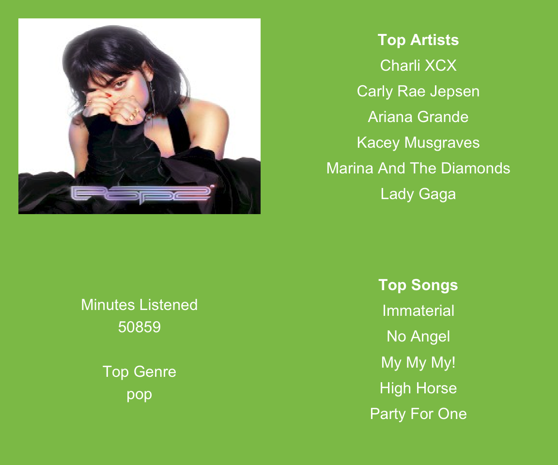
minutes <- as_ggplot(text_grob(paste("Minutes Listened", toString(round(mins)), "", "Top Genre", toString(topGenres[1, 1]), sep = "\n"), color = "white")) + bgTheme
img <- readPNG("images/albums.png")
im_A <- ggplot() +
background_image(img[1:250, 1:250, 1:3]) +
theme(plot.margin = margin(t = .5, l = .5, r = .5, b = .5, unit = "cm")) +
bgTheme
ggarrange(im_A, artistTable, minutes, trackTable, ncol = 2, nrow = 2)