My lab at Northwestern sits in a building near Lakeside Field, home to the school field hockey team. The team is quite sucessful: they won the national championship in 2021 and were runners-up in 2022. The team is once again in the hunt for the national championship in 2023, and I thought it would be fun to try to predict the outcome of the tournament (or at least quantify their odds).
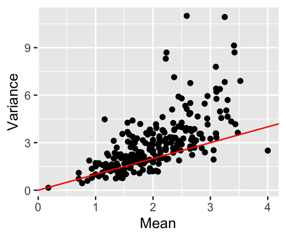
Figure 1
To do so, I build on some existing models built over the last half-century. To start, I create a model similar to Maher (1982), who uses the Poisson distribution to model the number of goals scored by each team. However, because the data are overdispursed (Figure 1), I use the negative binomial distribution instead.
The Model
The Poisson distribution represents the probability of a number of events occurring over a fixed period of time. In this case, we are interested in goals during the course of a game, which varies based on team ability. The Poisson distribution can be considered a special case of the negative binomial distribution when the mean is equal to the variance. Since this is not the case with the field hockey goals data, we use the negative binomial distribution instead. We consider the amount of scoring as a function of both a team’s offensive skill and the defensive skill of their opponent and additionally consider home field advantage.
model_formula<-bf(gf~1+# intercepthome+# home field advantage(1|team_id)+# offense(1|opponent)+# defenseoffset(log(match_time)),# overtime adjustment center=TRUE)
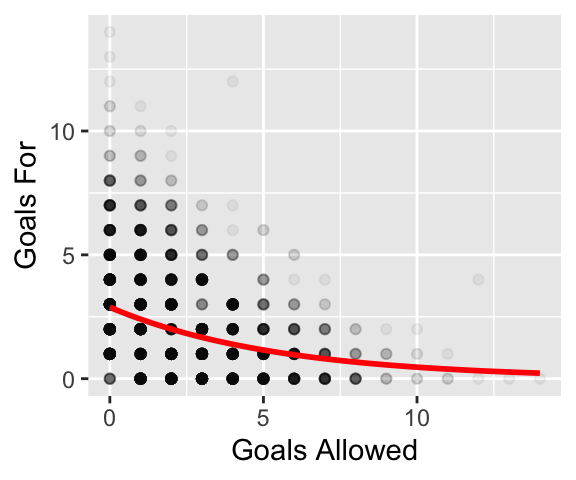
The simple model above assumes that the goals scored by each team are independent. This assumption, however, misses something we can see in our data: the number of goals scored by one team is negatively correlated with the number of goals scored by the other team (Figure 2). In fact, the probability of a shutout increases as a team scores more goals (or rather, teams that score more goals are more likely to get shutouts proportionally).
References
Maher, Michael J. 1982. “Modelling Association Football Scores.”Statistica Neerlandica 36 (3): 109–18.
Source Code
---title: "A Bayesian Model for NCAA Field Hockey"description: "Approximating skill and predicting outcomes with the negative binomial distribution"date: 2023-11-08bibliography: references.bibcategories: - R - Stan - brmsexecute: echo: false warning: false cache: true---```{r, setup, include=FALSE}```My lab at Northwestern sits in a building near Lakeside Field, home to the school field hockey team. The team is quite successful: they won the national championship in 2021 and were runners-up in 2022. The team is once again in the hunt for the national championship in 2023, and I thought it would be fun to try to predict the outcome of the tournament (or at least quantify their odds).```{r libraries-data, warning=FALSE, message=FALSE}library(tidyverse)library(arrow)library(brms)library(tidybayes)library(cfbplotR)library(ggtext)library(glue)library(grid)load_matches_year <-function(year) {read_feather(glue::glue("data/matches_{year}.feather")) %>%mutate(minutes =as.integer(stringr::str_extract(time, "\\d+(?=:)")),seconds =as.integer(stringr::str_extract(time, "(?<=:)\\d+")) ) %>%mutate(quarters = (minutes + seconds/60.0) /15.0) %>%mutate(match_time = quarters/4.0) %>%mutate(season=year)}# TODO: Some of these are missing times?matches <-c(2022, 2023, 2024) %>%map(load_matches_year) %>%bind_rows() %>%arrange(desc(home), date) %>%mutate(home_team = (home ==1))teams <- matches %>% dplyr::select(team_id, name) %>%distinct() %>%mutate(team_id =as.integer(team_id))``````{r}#| label: fig-poisson#| column: margin#| fig-width: 3#| fig-height: 2.5matches %>%group_by(team_id, season) %>%summarize(mean =mean(gf),var =var(gf) ) %>%ggplot(aes(x=mean, y=var)) +geom_point() +geom_abline(slope=1, intercept=0, color="red") +labs(x="Mean", y="Variance")```To do so, I build on some existing models built over the last half-century. To start, I create a model similar to @maher1982modelling, who uses the Poisson distribution to model the number of goals scored by each team. However, because the data are overdispersed (@fig-poisson), I use the negative binomial distribution instead.# The ModelThe Poisson distribution represents the probability of a number of events occurring over a fixed period of time. In this case, we are interested in goals during the course of a game, which varies based on team ability. The Poisson distribution can be considered a special case of the negative binomial distribution when the mean is equal to the variance. Since this is not the case with the field hockey goals data, we use the negative binomial distribution instead. We consider the amount of scoring as a function of both a team's offensive skill and the defensive skill of their opponent and additionally consider home field advantage.$$\text{goals}_{ij} \sim \text{NegBinom}(\alpha + \text{offense}_i + \text{defense}_j + \text{home})$$where:- $\text{goals}_{ij}$ is the number of goals scored by team $i$ against team $j$- $\alpha$ is an intercept term- $\text{offense}_i$ is the offensive skill of team $i$- $\text{defense}_j$ is the defensive skill of team $j$- $\text{home}$ is the home field advantageTo get the model to converge, we add the additional zero-sum constraints$$\sum_{i=1}^{n} \text{offense}_i = \sum_{i=1}^{n} \text{defense}_j = 0$$In `brms`, this model is specified as```{r}#| label: model-formula#| echo: truemodel_formula <-bf( gf ~1+# intercept home +# home field advantage (1| team_id) +# offense (1| opponent) +# defenseoffset(log(match_time)),# overtime adjustmentcenter=TRUE)``````{r, poisson-model}build_model <-function(matches) {brm( model_formula,data = matches,family =negbinomial(),cores =4,iter =2500,warmup =1500, )}model_2024 <-build_model((matches %>%filter(season ==2024) %>%filter(date <"11/08/2023")))model_2023 <-build_model((matches %>%filter(season ==2023)))model_2022 <-build_model((matches %>%filter(season ==2022)))```## Metrics and Visualization```{r}#| label: plot-offense-defenseoffense_defense <-function(model) { offense <- model %>%spread_draws(r_team_id[team_id,]) %>%group_by(team_id) %>%summarize(mean =mean(r_team_id),lower =quantile(r_team_id, 0.025),upper =quantile(r_team_id, 0.975) ) %>%arrange(desc(mean)) %>%left_join(teams, by ="team_id") defense <- model %>%spread_draws(r_opponent[opponent,]) %>%group_by(opponent) %>%summarize(mean =mean(r_opponent),lower =quantile(r_opponent, 0.025),upper =quantile(r_opponent, 0.975) ) %>%arrange(mean) %>%rename(team_id = opponent) %>%left_join(teams, by ="team_id") team_rename <-c("UAlbany"="Albany","App State"="Appalachian State","American"="American University","Boston U."="Boston University","Ohio St."="Ohio State","Penn St."="Penn State","Penn"="Pennsylvania","Massachusetts"="UMass","Ball St."="Ball State","Central Mich."="Central Michigan","Michigan St."="Michigan State","LIU"="Long Island University","Kent St."="Kent State" ) plot_data <-inner_join( (offense %>% dplyr::select(team_id, mean, name) %>%rename(offense=mean)), (defense %>% dplyr::select(team_id, mean) %>%rename(defense=mean)),by="team_id") %>%mutate(name =coalesce(team_rename[name], name)) %>%mutate(has_image = (name %in%valid_team_names())) %>%mutate(defense=-defense)return(plot_data)}plot_offense_defense <-function(plot_data) { plot <- plot_data %>%filter(has_image) %>%ggplot(aes(y=defense, x=offense, label=name, team=name)) +#geom_richtext(angle=-45) +geom_cfb_logos(width =0.05, angle=-45) +coord_fixed(ratio=1, xlim=c(-1.5, 1.5), ylim=c(-1.5, 1.5)) +labs(#title="2023-2024 NCAA Field Hockey Efficiency",x="Offense",y="Defense" ) +theme_bw() +theme(axis.title.x =element_text(angle =-45, hjust =0.5, vjust =0.5),axis.title.y =element_text(angle =-45, hjust =0.5, vjust =0.5),axis.text.x =element_blank(),axis.ticks.x =element_blank(),axis.text.y =element_blank(),axis.ticks.y =element_blank() ) grid::grid.newpage() vp <- grid::viewport(name ="rotate", y=0.4, angle =45, width =0.75, height =0.75) grid::pushViewport(vp)print(plot, vp="rotate", newpage =FALSE)}```::: panel-tabset### 2023```{r}#| label: offense-defense-2024#| fig-width: 6#| fig-height: 6#| classes: preview-imageod_2024 <-offense_defense(model_2024)plot_offense_defense(od_2024)```### 2022```{r}#| label: offense-defense-2023#| fig-width: 6#| fig-height: 6od_2023 <-offense_defense(model_2023)plot_offense_defense(od_2023)```### 2021```{r}#| label: offense-defense-2022#| fig-width: 6#| fig-height: 6od_2022 <-offense_defense(model_2022)plot_offense_defense(od_2022)```:::## Simulations```{r}draws <- model_2024 %>%spread_draws(b_Intercept, shape, b_home, r_team_id[team_id,], r_opponent[opponent,])``````{r}#| label: simulate-goalssimulate_goals <-function(draws, is_home, t1, t2) { draws %>%filter(team_id == t1) %>%filter(opponent == t2) %>%mutate(mu =exp(b_Intercept + r_team_id + r_opponent + b_home*is_home)) %>%rowwise() %>%mutate(goals =list(rnbinom(100, size=shape, mu=mu)),# TODO: how to do this with negative binomial?time =list(rgeom(100, 1- shape/(shape+mu)) / shape) ) %>%select(goals, time) %>%unnest(cols =c(goals, time))}``````{r}tournament_teams_list <-c("North Carolina","Northwestern","Duke","Maryland","Virginia","Liberty","Iowa","Rutgers","Harvard","Louisville","Syracuse","Saint Joseph's","Old Dominion","American","Miami (OH)","William & Mary")home_advantage <-c(1, 5, 5, 5, 17, 17, 17, 17, 17, 17, 17, 17, 17, 17, 17, 17)tournament_teams <-data.frame(name=tournament_teams_list,home=home_advantage ) %>%inner_join(teams, by="name") %>%mutate(seed=seq_along(name))``````{r}teams_win_percentage <-function(draws, home, t1, t2) { sim_1 <-simulate_goals(draws, home, t1, t2) sim_2 <-simulate_goals(draws, -home, t2, t1) goal_diff <- sim_1$goals - sim_2$goals first_rate <- sim_1$time < sim_2$time overtime_win <- (first_rate & (goal_diff ==0) & (pmin(sim_1$time, sim_2$time) < (1/3)))# TODO: Assume random for now shootouts <-sum((goal_diff ==0) & (pmin(sim_1$time, sim_2$time) >= (1/3))) shootout_win <-runif(shootouts) <0.5# TODO: Ignores shootout for now.# Could factor in when the rate is lower than 20return((sum(goal_diff >0) +sum(overtime_win) +sum(shootout_win)) /length(goal_diff))}``````{r, eval=FALSE}teams_win_percentage(draws, -1, 457, 509)``````{r}tournament_draws <- draws %>%filter(team_id %in% tournament_teams$team_id) %>%filter(opponent %in% tournament_teams$team_id)m <-matrix(0, nrow=nrow(tournament_teams), ncol=nrow(tournament_teams))for (i in1:(nrow(tournament_teams) -1)) {for (j in (i +1):nrow(tournament_teams)) { has_home_advantage <- tournament_teams$home[i] <= j win_percentage <-teams_win_percentage( tournament_draws,as.integer(has_home_advantage), tournament_teams$team_id[i], tournament_teams$team_id[j] ) m[i, j] <- win_percentage m[j, i] <-1- win_percentage }}``````{r}#| label: tournament-simulationtournament_round <-function(mat, teams) {if (length(teams) ==1) {return(teams[1]) }if (length(teams) ==2) { t1 <- teams[1] t2 <- teams[2]return(ifelse(runif(1) < mat[t1, t2], t1, t2)) } half_length <-length(teams) %/%2 first_half_winner <-tournament_round(mat, teams[1:half_length]) second_half_winner <-tournament_round(mat, teams[(half_length +1):length(teams)])return(tournament_round(mat, c(first_half_winner, second_half_winner)))}``````{r}y <-replicate(100000, tournament_round( m,seq(1, nrow(tournament_teams), 1))) %>%table() %>%prop.table() %>%as.data.frame() %>%setNames(c("s", "wins")) %>%mutate(seed =as.integer(s)) %>%inner_join(tournament_teams, by="seed") %>%arrange(desc(wins))y %>%mutate(winsp = wins*100) %>% dplyr::select(name, seed, winsp) %>% knitr::kable(digits=2, col.names=c("Team", "Seed", "Champs %"))```## Too simple?```{r}#| label: fig-goal-correlation#| column: margin#| fig-width: 3#| fig-height: 2.5matches %>%ggplot(aes(x=ga, y=gf)) +geom_point(alpha=0.05) +geom_smooth(method ="glm", method.args =list(family ="poisson"), se =FALSE, color ="red") +labs(x="Goals Allowed", y="Goals For")```The simple model above assumes that the goals scored by each team are independent. This assumption, however, misses something we can see in our data: the number of goals scored by one team is *negatively correlated* with the number of goals scored by the other team (@fig-goal-correlation). In fact, the probability of a shutout *increases* as a team scores more goals (or rather, teams that score more goals are more likely to get shutouts proportionally).```{r, eval=FALSE}model_2024 <-build_model((matches %>%filter(season ==2024)))draws <- model_2024 %>%spread_draws(b_Intercept, shape, b_home, r_team_id[team_id,], r_opponent[opponent,])tournament_teams_list <-c("North Carolina","Northwestern","Duke","Virginia")home_advantage <-c(1, 5, 5, 5)tournament_teams <-data.frame(name=tournament_teams_list,home=home_advantage ) %>%inner_join(teams, by="name") %>%mutate(seed=seq_along(name))``````{r, bivariate-model, eval=FALSE}teams <- matches_2023 %>% dplyr::select(team_id, name) %>%distinct() %>%mutate(team_id =as.integer(team_id))data <- matches_2023 %>%# TODO: At the moment, matches are counted twice... #mutate(i = paste(date, pmin(team_id, opponent), pmax(team_id, opponent))) %>% #distinct(i, .keep_all=T) %>%arrange(date) %>%drop_na() %>%mutate(season=2022) %>% dplyr::select(season, team_id, opponent, gf, ga) %>%mutate(team_id =as.integer(team_id)) %>%inner_join(teams, by=c("team_id"="team_id")) %>%rename(team_id="team_id", home="name") %>%mutate(opponent =as.integer(opponent)) %>%inner_join(teams, by=c("opponent"="team_id")) %>%rename(opponent="opponent", away="name") %>%select(season, home, away, gf, ga)sf <-stan_foot(data=data,model="double_pois",ind_home="FALSE",predict=2)```