Carl Colglazier – Building an intuition for the kelly criterion

Motivating Example

In an experiment, participants got a bankroll of $25 and a coin, weighted such that it landed on heads 60% of the time (Haghani and Dewey 2017). Over the course of the next 30 minutes, they could bet up to their entire bankroll on coin flips.

Despite the odds being heavily on their side, more than a quarter of participants lost their initial bankroll and more than a third lost money. How? Most players ended playing very bad strategies. Many even bet their entire bankroll on a single flip!

You can try out this senario in the interactive below. The slider controls the percentage of your bankroll you bet on each flip.

function prob_to_odds(p) {
  return (1 - p) / p
}

function kelly_criterion(prob_win, p_odds) {
  let b = prob_to_odds(p_odds)
  return (prob_win * b - (1 - prob_win)) / b
}

viewof betsize = Inputs.range(
  [0, 100], 
  {value: 50, step: 1, label: "Bet size (%):"}
)

array = [25.0, 25.0, 25.0];

viewof addButton = {
  // Create an HTML button element
  const button = html`<button>Bet</button>`;
  // Define what happens when you click the button
  button.onclick = () => {
    let bankroll = 25
    if (array.length > 0) {
      bankroll = array[array.length - 1];
    }
    let win = Math.random() < 0.6 ? 1 : -1;
    let update = bankroll + (betsize / 100) * bankroll * win;
    array.push(update); // For example, add a random number to the array
    // Log the array to the console or update the display
    console.log(array, bankroll, win, update);
  };
  
  return button;
}

viewof resetButton = {
  // Create an HTML button element
  const rbutton = html`<button>Start over</button>`;
  // Define what happens when you click the button
  rbutton.onclick = () => {
    array.length = 0;
    array.push(25.0);
  };
  return rbutton;
}

arrayDisplay = {
  // Wait for the button to be clicked
  addButton;
  resetButton;
  // Return the array for display
  return array;
}

arrayDisplay[arrayDisplay.length - 1];

function simulation(betsize) {
  var data = [];
  var bankroll = 25.0;
  for (var i = 0; i < 250; i++) {
    var bet = (betsize / 100) * bankroll;
    if (Math.random() < 0.6) {
      bankroll += bet;
    } else {
      bankroll -= bet;
    }
    data.push({"time": i, "bankroll": bankroll})
  }
  return data
}
data = arrayDisplay.map((y,i) => {
  let data = {};
  data["time"] = i;
  data["value"] = y; 
  return data;
});
//simulation(betsize);
Plot.plot({
  marks: [
    Plot.lineY(data, {x: "time", y: "value"})
  ]
})

Defining the Kelly Criterion

The Kelly criterion describes an optimal betting size strategy which maximizes the expected growth rate (by optimizing the expected value of the logarithm of wealth). In the long run, it is the optimal strategy (e.g. as the number of bets approaches infinity).

\[ f\ast = p - \frac{1-p}{b} \]

where

$f\ast$ is the fraction to bet
$p$ is the expected probability the event occurs (and $1 - p$ is the probability it does not occur), and
$b$ is odds, or the proportion gained from the bet.

The Kelly criteron tells us to bet when $b > \frac{1-p}{p}$, or when the payout is greater than the odds the event occurs.

Origins

Kelly (1956) describes his criterion through the lens of information theory. In his original paper, he presents an example of a gambler with a private wire which gives them insight into the results of a series of baseball games between evenly matched teams. The wire is noisy, and the gambler can only correctly predict the outcome of a game with probability $p$. If the wire was perfect, the gambler could simply bet their entire bankroll each time and grow their bankroll with $N$ bets to $2^N$ times the original bankroll; however, because the wire is noisy, the gambler must bet less than their entire bankroll to avoid going bust (Kelly 1956, 918–19). How much should they bet?

Kelly suggests that we maximize the expected value of the logorithm of wealth. We can express this as the growth rate $r$ using the same notation:

\[r = (1 + fb)^p \cdot (1 - fb)^{(1-p)}\]

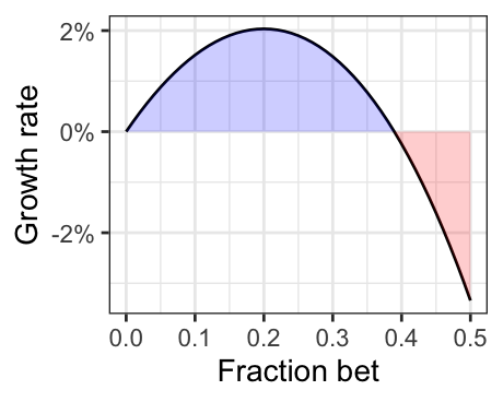
Figure 1: Growth rate for a bet with +100 odds and p=0.6

To gain an intuition for the problem, we can plot out all the possible growth rates for a bet with +100 odds and $p=0.55$ as we have in Figure 1.

To optimize $r$, it is easiest to take the derivative, but first we can get rid of the exponents by taking the log of both sides:

\[\log(r) = p\log(1 + fb) + (1-p)\log(1 - fb)\]

When the derivative of this expression is zero, we have found the maximum logarithm of the growth rate.¹ The use of the logirthm as the value function is somewhat arbitrary and likely has a lot to do with the criterion’s origins in information theory. Kelly (1956) himself notes: “The reason has nothing to do with the value function which he attached to his money, but merely with the fact that it is the logarithm which is additive in repeated bets and to which the law of large numbers applies” (Kelly 1956, 925–26). Kelly describes how a gambler should deviate their strategy from his criterion: if they have a different value function, they could use a different strategy.

¹ See the Wikipedia page on the Kelly criterion for the full proof.

I should note that the Kelly criterion was created for a situation with a lot of assumptions. Among them:

The gambler knows the true probability of the event occurring.
The gambler has infinite repeated bets.
The gambler’s only goal is to maximize their bankroll.
The gambler can bet as much or as little as they want every time.
Opportunity costs are unimportant.

The Kelly criterion is a useful heuristic, but few of these assumptions hold up in real life.

Probability and bet sizes

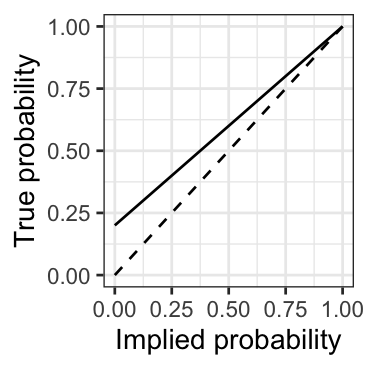
Figure 2: Edge needed to bet 20% of bankroll

The logarithmic properties of the Kelly criterion lead to some desirable outcomes. For instance, given even odds (+100) the criterion tells us we need a 60% winning expectation (20% EV) to bet 20% of our bankroll, but at longer odds like +400, we would need to expect to win 36% of the time (80% EV). Thus the Kelly criterion suggests we need a higher expectation of our edge to bet more on bets with long odds. However, with -300 odds, we’d need to expect to win 80% of the time (6.6–6.7% EV) to bet 20% of our bankroll. This is a much lower edge required for a bet with a high probability of winning.

Bet size	True probability	Payout	Edge	Implied probability
20%	30%	700	140.0%	12%
20%	40%	300	60.0%	25%
20%	50%	167	33.3%	37%
20%	60%	-100	20.0%	50%
20%	70%	-167	12.0%	62%
20%	80%	-300	6.7%	75%
20%	90%	-700	2.9%	88%

A typical gambler may not only want to maximize bankroll size, but also minimize the chance of losing all their money by going bust. Here, the relationship between probability and the size of bets remains important.

Let us say we know we have a consistent, unwaiving 2% edge on a repeated set of bets. Table 1 shows the bet sizes for a set of gamblers each betting with this edge at different odds. Note that the bet size increases with the probability of the bets winning.

Payout	Implied probability	True probability	Bet size
900	10.0%	10.2%	0.2%
400	20.0%	20.4%	0.5%
233	30.0%	30.6%	0.9%
150	40.0%	40.8%	1.3%
100	50.0%	51.0%	2.0%
-150	60.0%	61.2%	3.0%
-233	70.0%	71.4%	4.7%
-400	80.0%	81.6%	8.0%
-900	90.0%	91.8%	18.0%

Table 1: Bet sizes for gamblers using the Kelly criterion each betting with a 2% edge with different odds

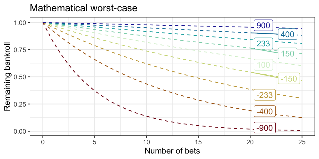
Imagine if all of these bettors became extremely unlucky and all of their bets lost. How much they lose is a function of how much they bet.

\[ (1-f\ast)^n \]

where $n$ is the number of bets.

We can simulate the scenario for each of the bettors in Table 1. As seen in Figure 3, given the same edge, the bettors with higher odds of winning can potentially lose their money the fastest. This is because they are betting more of their bankroll each time.

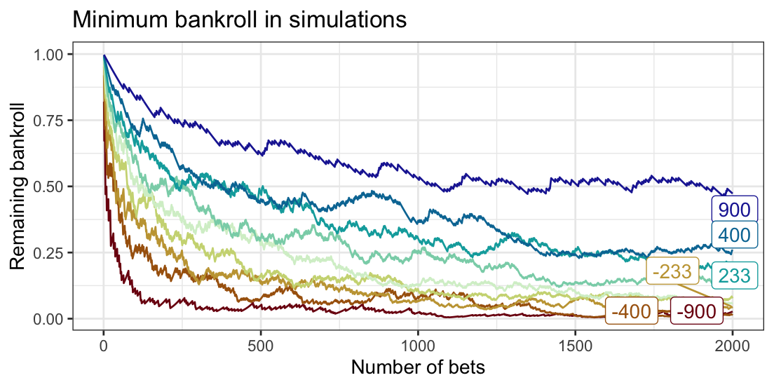
While, the worst-case scenaio is within the bounds of the possible, it’s not exactly likely. To give an idea for the range of outcomes, we can simulate how the bettors in Table 1 might fare. To reduce the effects of random chance, we can aggregate over 1,000 simulations. Here, the same pattern emerges where the bets on higher probability events can lose money quickest, but the worst-case simulated events rarely approach the worst-case over time (losing 2000 bets is unlikely even if you only have a 10% of each bet winning).

Figure 5: On average, bets with higher odds make more money given the same percentage of expected value

If there is so much risk involved with betting big bankrolls on higher probability events, why does Kelly tell us to do it? As it turns out, it is very profitable. Figure 5 shows that the big bets by far return the highest profit over time. I had to change the scale to $\log10$ becasue the difference is so dramatic.

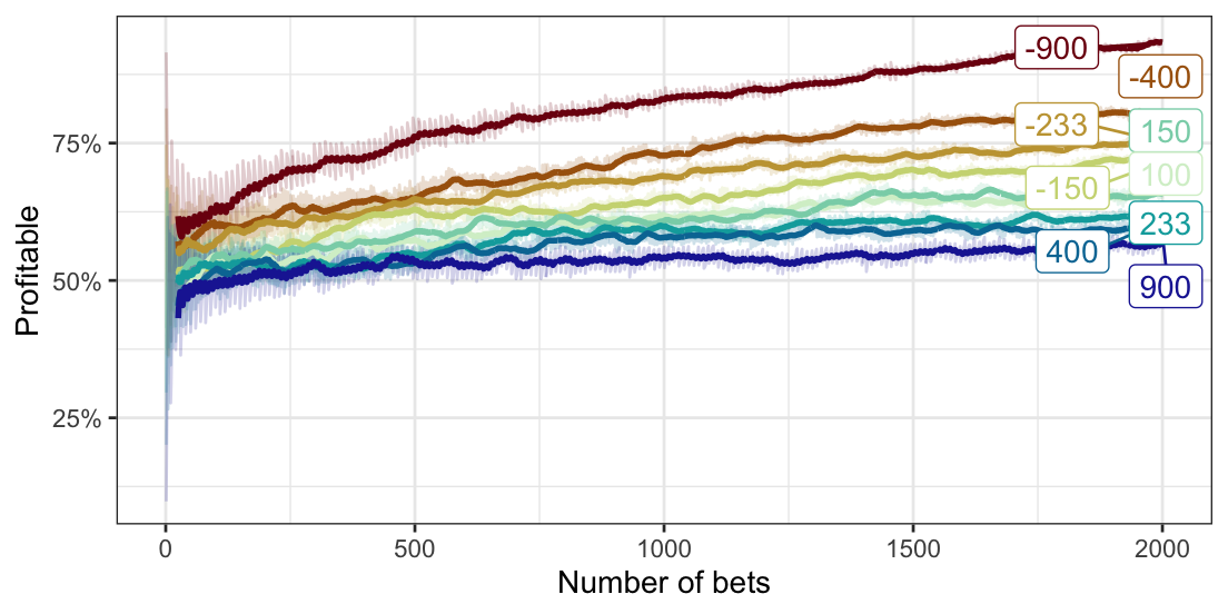
And it’s not just the median. Over the same number of bets, those betting on higher probability events are more likely to make a profit. It pays to bet big! And over time, many of the unlukcy bettors get less unlucky and end up making a profit.

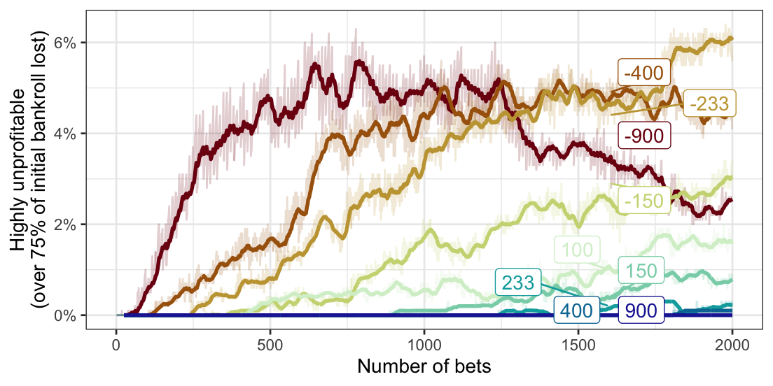
There are two things going on in these simulations:

Higher probability bets make more profit in aggregate.
Higher probability bets create higher variance in their outcomes, so when they lose, they lose a lot.

The variance of bankrolls increases with the number of bets

Final Thoughts

The Kelly criterion is effective in cases where you goals align with optimizing the logarithm of the rate growth of wealth (which seems true in many cases) and where the assumptions don’t seem too outlandish given your information.

References

Haghani, Victor, and Richard Dewey. 2017. “Rational Decision Making Under Uncertainty: Observed Betting Patterns on a Biased Coin.” Journal of Portfolio Management 43 (3): 2–8. https://doi.org/10.3905/jpm.2017.43.3.002.

Kelly, John L. 1956. “A New Interpretation of Information Rate.” The Bell System Technical Journal 35 (4): 917–26.

--- title: "Building an intuition for the kelly criterion" description: "Simulating an effective bankroll management strategy" author: "Carl Colglazier" date: 2023-11-03 bibliography: "references.bib" categories: - information theory #freeze: false fig-width: 6 fig-height: 4.5 fig-dpi: 92 format: html: fig-cap-location: bottom execute: echo: false output: true warning: false --- ```{r} #| label: setup library(tidyverse) library(arrow) library(knitr) library(scales) library(ggrepel) library(geomtextpath) library(tidyquant) library(gganimate) library(colorspace) plot_theme <- theme_bw() + theme(legend.position = "none") theme_set(plot_theme) ``` ## Motivating Example In an experiment, participants got a bankroll of \$25 and a coin, weighted such that it landed on heads 60% of the time [@haghani2017]. Over the course of the next 30 minutes, they could bet up to their entire bankroll on coin flips. Despite the odds being heavily on their side, more than a quarter of participants lost their initial bankroll and more than a third lost money. How? Most players ended playing very bad strategies. Many even bet their entire bankroll on a single flip! You can try out this senario in the interactive below. The slider controls the percentage of your bankroll you bet on each flip. ```{ojs} function prob_to_odds(p) { return (1 - p) / p } function kelly_criterion(prob_win, p_odds) { let b = prob_to_odds(p_odds) return (prob_win * b - (1 - prob_win)) / b } ``` ::: column-page ```{ojs} //| label: cointoss-simulation-inputs //| panel: sidebar viewof betsize = Inputs.range( [0, 100], {value: 50, step: 1, label: "Bet size (%):"} ) array = [25.0, 25.0, 25.0]; viewof addButton = { // Create an HTML button element const button = html`<button>Bet</button>`; // Define what happens when you click the button button.onclick = () => { let bankroll = 25 if (array.length > 0) { bankroll = array[array.length - 1]; } let win = Math.random() < 0.6 ? 1 : -1; let update = bankroll + (betsize / 100) * bankroll * win; array.push(update); // For example, add a random number to the array // Log the array to the console or update the display console.log(array, bankroll, win, update); }; return button; } viewof resetButton = { // Create an HTML button element const rbutton = html`<button>Start over</button>`; // Define what happens when you click the button rbutton.onclick = () => { array.length = 0; array.push(25.0); }; return rbutton; } arrayDisplay = { // Wait for the button to be clicked addButton; resetButton; // Return the array for display return array; } arrayDisplay[arrayDisplay.length - 1]; ``` ```{ojs} //| label: cointoss-simulation-output //| panel: fill function simulation(betsize) { var data = []; var bankroll = 25.0; for (var i = 0; i < 250; i++) { var bet = (betsize / 100) * bankroll; if (Math.random() < 0.6) { bankroll += bet; } else { bankroll -= bet; } data.push({"time": i, "bankroll": bankroll}) } return data } data = arrayDisplay.map((y,i) => { let data = {}; data["time"] = i; data["value"] = y; return data; }); //simulation(betsize); Plot.plot({ marks: [ Plot.lineY(data, {x: "time", y: "value"}) ] }) ``` ::: ## Defining the Kelly Criterion The Kelly criterion describes an optimal betting size strategy which maximizes the expected *growth rate* (by optimizing the expected value of the logarithm of wealth). In the *long run*, it is the optimal strategy (e.g. as the number of bets approaches infinity). $$ f\ast = p - \frac{1-p}{b} $$ where - $f\ast$ is the fraction to bet - $p$ is the expected probability the event occurs (and $1 - p$ is the probability it does not occur), and - $b$ is odds, or the proportion gained from the bet. The Kelly criteron tells us to bet when $b > \frac{1-p}{p}$, or when the payout is greater than the odds the event occurs. ## Origins @kelly1956new describes his criterion through the lens of information theory. In his original paper, he presents an example of a gambler with a private wire which gives them insight into the results of a series of baseball games between evenly matched teams. The wire is noisy, and the gambler can only correctly predict the outcome of a game with probability $p$. If the wire was perfect, the gambler could simply bet their entire bankroll each time and grow their bankroll with $N$ bets to $2^N$ times the original bankroll; however, because the wire is noisy, the gambler must bet less than their entire bankroll to avoid going bust [@kelly1956new, 918-919]. How much should they bet? Kelly suggests that we maximize the expected value of the logorithm of wealth. We can express this as the growth rate $r$ using the same notation: $$r = (1 + fb)^p \cdot (1 - fb)^{(1-p)}$$ ```{r} #| label: fig-growth-rate #| column: margin #| fig-width: 2.5 #| fig-height: 2 #| fig-cap: Growth rate for a bet with +100 odds and p=0.6 kelly_oh_six <- function(x, b, p) { (1 + b*x)^p * (1 - x)^(1-p) - 1.0 } b <- 1.0 p <- 0.6 formula_data <- tibble(f = seq(0, 0.5, 0.01), b=b, p=p) %>% mutate( r = kelly_oh_six(f, b, p=p) ) kelly_b <- function(x) kelly_oh_six(x, b=b, p=p) stop_point <- uniroot(kelly_b, c(0.01, 1))$root formula_data %>% ggplot(aes(x=f, y=r)) + geom_line() + ylab("Growth rate") + xlab("Fraction bet") + scale_y_continuous(labels = scales::percent_format()) + stat_function( fun = kelly_b, xlim=c(0, stop_point), geom = "area", fill = "blue", alpha = 0.2 ) + stat_function( fun = kelly_b, xlim=c(stop_point, max(formula_data$f)), geom = "area", fill = "red", alpha = 0.2 ) + plot_theme ``` To gain an intuition for the problem, we can plot out all the possible growth rates for a bet with +100 odds and $p=0.55$ as we have in @fig-growth-rate. To optimize $r$, it is easiest to take the derivative, but first we can get rid of the exponents by taking the log of both sides: $$\log(r) = p\log(1 + fb) + (1-p)\log(1 - fb)$$ When the derivative of this expression is zero, we have found the maximum logarithm of the growth rate.[^1] The use of the logirthm as the value function is somewhat arbitrary and likely has a lot to do with the criterion's origins in information theory. @kelly1956new himself notes: "The reason has nothing to do with the value function which he attached to his money, but merely with the fact that it is the logarithm which is additive in repeated bets and to which the law of large numbers applies" [@kelly1956new, 925-926]. Kelly describes how a gambler should deviate their strategy from his criterion: if they have a different value function, they could use a different strategy. [^1]: See the [Wikipedia page on the Kelly criterion](https://en.wikipedia.org/wiki/Kelly_criterion) for the full proof. I should note that the Kelly criterion was created for a situation with a lot of assumptions. Among them: 1. The gambler knows the true probability of the event occurring. 2. The gambler has infinite repeated bets. 3. The gambler's only goal is to maximize their bankroll. 4. The gambler can bet as much or as little as they want every time. 5. Opportunity costs are unimportant. The Kelly criterion is a useful heuristic, but few of these assumptions hold up in real life. ## Probability and bet sizes ```{r} #| label: fig-betsize-edge #| column: margin #| fig-width: 2 #| fig-height: 2 #| fig-cap: Edge needed to bet 20% of bankroll kelly_criterion <- function(p, b) { p - (1-p)/b } implied_prob_from_edge <- function(edge, p) { p + p*edge } expected_value <- function(p, b) { p*b - (1-p) } convert_to_american_odds <- function(odds) { if(odds >= 1) { return((odds) * 100) } else { return(-100 / (odds)) } } bet_size <- 0.2 formula_data <- tibble(betsize=bet_size, p=seq(bet_size, 1.0, 0.01),) %>% mutate(b=((1-p)/(p-betsize))) %>% mutate(ev=b*betsize) %>% mutate(implied=1/(b+1)) formula_data %>% ggplot(aes(x=implied, y=p)) + stat_function(fun=function(x) {x}, geom="line", linetype="dashed") + geom_line() + xlim(0.0, 1.0) + ylim(0.0, 1.0) + labs( x="Implied probability", y="True probability", ) ``` The logarithmic properties of the Kelly criterion lead to some desirable outcomes. For instance, given even odds (+100) the criterion tells us we need a 60% winning expectation (20% EV) to bet 20% of our bankroll, but at longer odds like +400, we would need to expect to win 36% of the time (80% EV). Thus the Kelly criterion suggests we need a higher expectation of our edge to bet more on bets with long odds. However, with -300 odds, we'd need to expect to win 80% of the time (6.6--6.7% EV) to bet 20% of our bankroll. This is a much lower edge required for a bet with a high probability of winning. ```{r} #| label: tbl-1 tibble(betsize=0.2, p=seq(0.3, 0.9, 0.1),) %>% mutate(b=((1-p)/(p-betsize))) %>% mutate(ev=b*betsize) %>% mutate(implied=1/(b+1)) %>% mutate(across(c(betsize, p, ev, implied), ~percent(.))) %>% mutate(b=sapply(b, convert_to_american_odds)) %>% kable(col.names=c("Bet size", "True probability", "Payout", "Edge", "Implied probability"), digits=0, align="rrrrr") ``` A typical gambler may not only want to maximize bankroll size, but also minimize the chance of losing all their money by going bust. Here, the relationship between probability and the size of bets remains important. Let us say we know we have a consistent, unwaiving 2% edge on a repeated set of bets. @tbl-betsizes shows the bet sizes for a set of gamblers each betting with this edge at different odds. Note that the bet size increases with the probability of the bets winning. ```{r} ev_amount <- 0.02 convert_to_american_odds_p <- function(p) { if (p > 0.5) { return(-100 * (p/(1-p))) } else { return(100 * ((1-p)/p)) } } convert_to_payouts <- function(p) { (1-p)/p } bettors <- tibble(given_p=seq(0.1, 0.9, 0.1)) %>% mutate(true_p=implied_prob_from_edge(ev_amount, given_p)) %>% mutate(payout=sapply(given_p, convert_to_american_odds_p)) %>% mutate(payout=round(payout)) %>% mutate(b=convert_to_payouts(given_p)) %>% mutate(betsize=kelly_criterion(true_p, b)) ``` ```{r} #| label: tbl-betsizes #| tbl-cap: "Bet sizes for gamblers using the Kelly criterion each betting with a 2% edge with different odds" #| tbl-cap-location: margin bettors %>% dplyr::select(payout, given_p, true_p, betsize) %>% mutate(across(c(given_p, true_p, betsize), ~percent(., accuracy=0.1))) %>% kable(col.names=c("Payout", "Implied probability", "True probability", "Bet size"), align="r") ``` Imagine if all of these bettors became extremely unlucky and all of their bets lost. How much they lose is a function of how much they bet. $$ (1-f\ast)^n $$ where $n$ is the number of bets. ```{r} #| label: run-simulations #| cache: true num_sims <- 1000 num_bets <- 2000 run_bets <- function(x, y) { x*y } simulate_bets <- function(df) { result <- tibble( time=1:num_bets, odds=df$payout, b=df$b, p=df$true_p, betsize=df$betsize, i=df$i ) result$win <- (runif(nrow(result)) < result$p) result <- result %>% mutate(w = ifelse(win, 1+betsize*b, 1-betsize)) %>% mutate(value=accumulate(w, run_bets, .init=1000)[-1]) return(result) } ids <- tibble(i=1:num_sims) sim_df <- bettors %>% mutate(id=row_number()) %>% uncount(num_sims, .id='rep_id') %>% mutate(i=(id-1)*num_sims+rep_id) %>% purrr::pmap(data.frame) %>% map_dfr(simulate_bets) ``` ```{r} df <- sim_df %>% mutate(odds=factor(odds)) %>% group_by(p, odds, time) %>% summarize( min=min(value), mean=mean(value), median=median(value), profitable=sum(value > 1000)/n(), highly_unprofitable=sum(value < 250)/n(), .groups = "drop" ) ``` We can simulate the scenario for each of the bettors in @tbl-betsizes. As seen in @fig-losses-1, given the same edge, the bettors with higher odds of winning can potentially lose their money the fastest. This is because they are betting more of their bankroll each time. While, the worst-case scenaio is within the bounds of the possible, it's not exactly likely. To give an idea for the range of outcomes, we can simulate how the bettors in @tbl-betsizes might fare. To reduce the effects of random chance, we can aggregate over 1,000 simulations. Here, the same pattern emerges where the bets on higher probability events can lose money quickest, but the worst-case simulated events rarely approach the worst-case over time (losing 2000 bets is unlikely even if you only have a 10% of each bet winning). ```{r} #| layout-ncol: 2 #| fig-width: 6 #| fig-height: 3 #| column: page #| fig-cap-location: bottom #| label: fig-losses n_bets_tibble <- tibble(n_bets=seq(0,25,1)) expand( bettors, nesting(payout, betsize), n_bets_tibble) %>% mutate(worst_case=(1-betsize)^n_bets) %>% mutate(odds=factor(payout)) %>% ggplot(aes(x=n_bets, y=worst_case, color=odds, label=odds)) + geom_line(linetype="dashed") + geom_label_repel(data=(. %>% filter(n_bets==20)), nudge_x = 0.35) + labs( title="Mathematical worst-case", x="Number of bets", y="Remaining bankroll" ) + plot_theme + scale_color_discrete_divergingx(palette="Roma") df %>% mutate(m=min/1000) %>% ggplot(aes(x=time, y=m, color=odds, label=odds)) + geom_line() + geom_label_repel(data=(. %>% filter(time==max(time))), nudge_x = 0.35) + labs( title="Minimum bankroll in simulations", x="Number of bets", y="Remaining bankroll" ) + plot_theme + scale_color_discrete_divergingx(palette="Roma") ``` ```{r} #| label: fig-median-bankroll #| column: margin #| fig-width: 2 #| fig-height: 2 #| fig-cap: "On average, bets with higher odds make more money given the same percentage of expected value" df %>% ggplot(aes(x=time, y=median, color=odds, label=odds)) + geom_line(alpha=0.2) + geom_ma(ma_fun = SMA, n = 50, linetype = 1, size = 1) + geom_label_repel(data=(. %>% filter(time==max(time))), nudge_x = 0.35) + ylab("Median bankroll") + xlab("Number of bets") + scale_y_log10() + plot_theme + scale_color_discrete_divergingx(palette="Roma") ``` If there is so much risk involved with betting big bankrolls on higher probability events, why does Kelly tell us to do it? As it turns out, it is very profitable. @fig-median-bankroll shows that the big bets by far return the highest profit over time. I had to change the scale to $\log10$ becasue the difference is so dramatic. And it's not just the median. Over the same number of bets, those betting on higher probability events are more likely to make a profit. It pays to bet big! And over time, many of the unlukcy bettors get less unlucky and end up making a profit. ```{r} #| layout-ncol: 2 #| fig-width: 6 #| fig-height: 3 #| column: page df %>% ggplot(aes(x=time, y=profitable, color=odds, label=odds)) + geom_line(alpha=0.2) + geom_ma(ma_fun = SMA, n = 25, linetype = 1, size = 1) + geom_label_repel(data=(. %>% filter(time==max(time))), nudge_x = 0.35) + scale_y_continuous(labels = scales::percent_format()) + ylab("Profitable") + xlab("Number of bets") + plot_theme + scale_color_discrete_divergingx(palette="Roma") df %>% ggplot(aes(x=time, y=highly_unprofitable, color=odds, label=odds)) + geom_line(alpha=0.2) + geom_ma(ma_fun = SMA, n = 25, linetype = 1, size = 1) + geom_label_repel(data=(. %>% filter(time==max(time)/1.25)), nudge_x = 0.35) + scale_y_continuous(labels = scales::percent_format()) + ylab("Highly unprofitable\n(over 75% of initial bankroll lost)") + xlab("Number of bets") + plot_theme + scale_color_discrete_divergingx(palette="Roma") ``` There are two things going on in these simulations: 1. Higher probability bets make more profit in aggregate. 2. Higher probability bets create higher variance in their outcomes, so when they lose, they lose a lot. ```{r} #| column: page-right #| fig-show: animate #| fig-cap: "The variance of bankrolls increases with the number of bets" #| cache: true #| animation-hook: ffmpeg #| ffmpeg-format: gif animation <- sim_df %>% filter(time <= 500) %>% filter(time %% 10 == 0) %>% mutate(result=log(value), odds=factor(odds)) %>% ggplot(aes(result, fill=odds, label=odds, group=odds)) + geom_histogram(bins=75, alpha=1.0, position = 'identity') + scale_x_continuous(labels = label_math(e^.x)) + facet_wrap(~odds) + plot_theme + scale_fill_discrete_divergingx(palette="Roma") + labs(title = 'Number of bets: {frame_time}', x="Bankroll") + transition_time(time) animate(animation, fps = 24, duration = 5) ```  ## Final Thoughts The Kelly criterion is effective in cases where you goals align with optimizing the logarithm of the rate growth of wealth (which seems true in many cases) and where the assumptions don't seem too outlandish given your information.