Efficiency models have had great success in predicting the outcomes of basketball games. The idea is simple: break everything down to possessions. Good teams score points on their possessions, while limiting opponents from scoring on their possessions. This basic principle underpins offensive and defensive ratings.
Just the raw numbers do not tell the whole story. The top scoring offense in 2025 was Murray State, the MVC champions ranked 185th in strength of schedule and whom the selection committee placed as an 11 seed; the top scoring defense in 2025 was 16 seed UNCG, ranked 244th in strength of schedule. It’s not just the totals: it’s also who you play against. A predictive model will need to be able to account for this.
Offensive and Defensive Rating Models
Everything goes back to possessions. For simplicity, I use a possession loss model, which Kubatko et al. (2007) define as1
1Oliver (2004) and his work popularized a number of statistical approaches to analyzing basketball
eff_form<-bf(efficiency|weights(weight)~1+home_off+(1|team_id)+(1|opponent_team_id), center =TRUE)prior<-c(prior(normal(1.0, 0.15), class ="Intercept"),prior(normal(0.1, 0.05), class ="b", coef ="home_off"),prior(cauchy(0, 2), class ="sd", group ="team_id"),prior(cauchy(0, 2), class ="sd", group ="opponent_team_id"),prior(cauchy(0, 1.5), class ="sigma"))bmodel<-brm( formula =eff_form, data =(team_game_data|>mutate(home_off =ifelse(home==1, 1, 0))), chains =5, iter =4000, warmup =2000, cores =5, file =here::here("notes/2025-wbb/data/eff_model2"), prior =prior)
Results
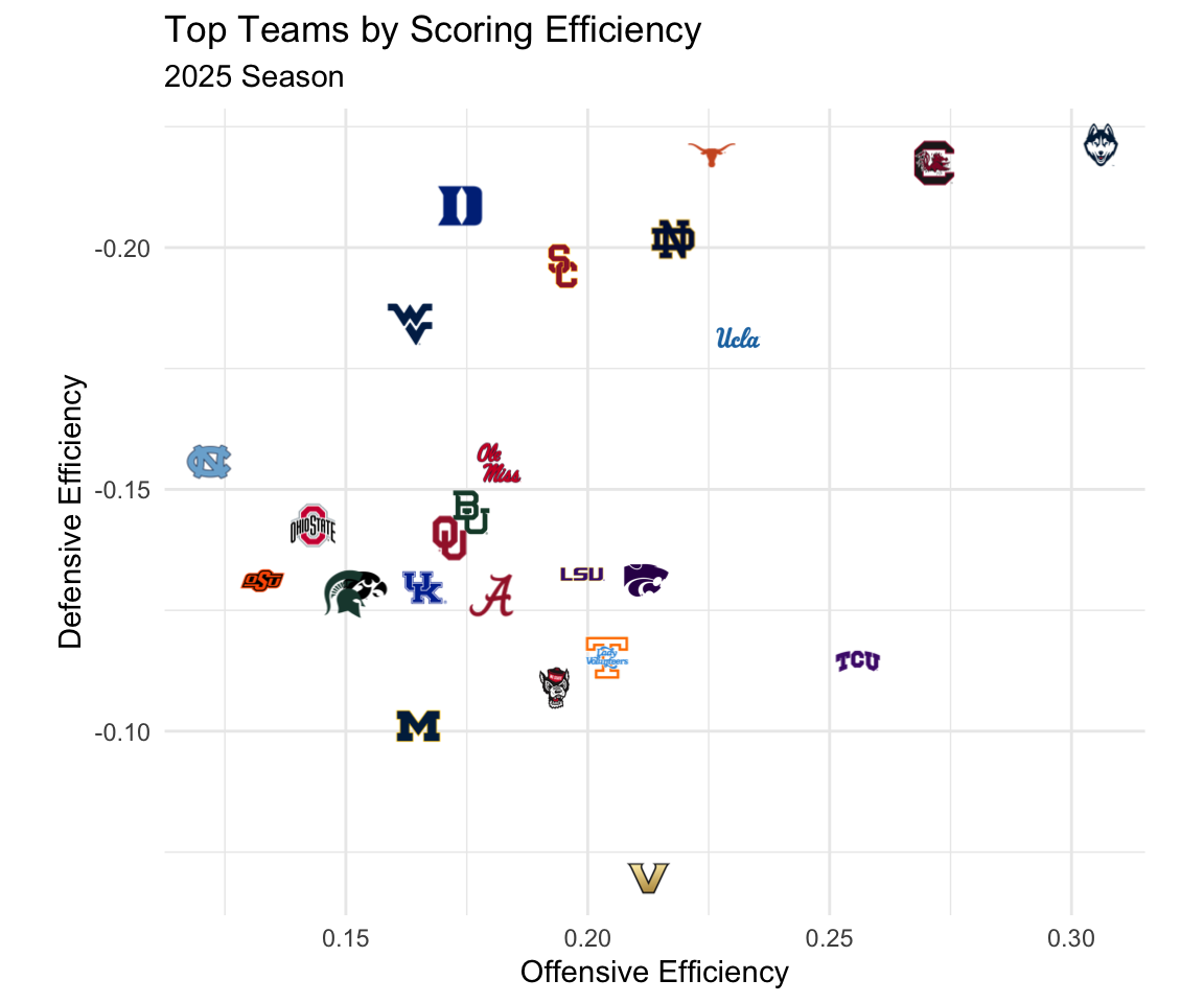
Figure 1: Offensive and defensive ratings for top teams in the NCAA women’s basketball tournament. Teams near the top right of the graph have the best overall ratings.
The raw offense and defense scores can be thought of as answering the question: on a given possession, how many more points does this team score on offense and limit on defense against an average team?
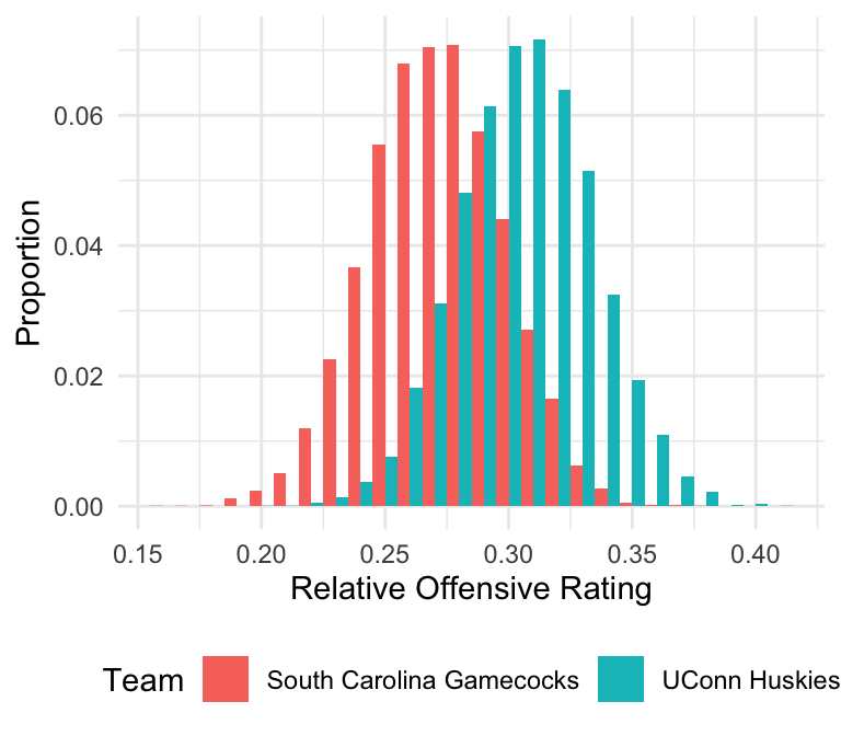
Because this is a Bayesian model, the posterior represents thousands of probable ways the relative strengths of the teams can explain the observed outcomes (scores from the games).
Table 1: Small sample of draws from the posterior for two teams.
Figure 2: Histogram of draws from the posterior for two teams’ relative offensive ratings.
There are a few ways we could consider what team is the “best” from this model:
What is the team’s average (mean and median) rank across the posterior draws?
What percentage of games would we expect each team to win against an average team?
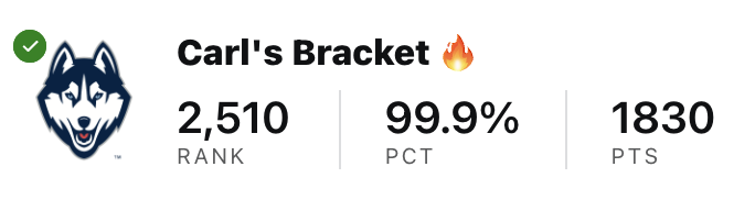
I used this model to help me create my bracket, ranking in the top 0.01% out of millions of submissions on ESPN. My bracket correctly predicted the national champion, the finals matchup, all four teams in the Final Four, 7/8 teams in the Elite Eight, and 15/16 teams in the Sweet Sixteen.
My final point total and rank on ESPN’s Tournament Challenge
References
Gilani, Saiem, and Geoffery Hutchinson. 2021. “Wehoop: Access Women’s Basketball Play by Play Data.”CRAN: Contributed Packages. The R Foundation. https://doi.org/10.32614/cran.package.wehoop.
Kubatko, Justin, Dean Oliver, Kevin Pelton, and Dan T Rosenbaum. 2007. “A Starting Point for Analyzing Basketball Statistics.”Journal of Quantitative Analysis in Sports 3 (3).
Oliver, Dean. 2004. Basketball on Paper: Rules and Tools for Performance Analysis. U of Nebraska Press.
Source Code
---title: Predicting the 2025 NCAA Division I Women's Basketball Tournament with a Multilevel Modeldescription: Using offensive and defensive ratings to simulate the odds of cutting down the netsdate: 2025-03-20bibliography: bibliography.bibtags: [sports, brms]format: html: code-fold: true html-table-processing: noneexecute: warning: false error: false echo: false---```{r}#| label: setuplibrary(tidyverse)library(brms)library(tidybayes)library(gt)library(furrr)# Tricks Positron to think we're RSTUDIO# Needed because of this issue:# https://github.com/posit-dev/positron/issues/5920Sys.setenv(RSTUDIO =1)game_weight <-function(days) {return(0.995^ days)}n_cores <-6my_gt_theme <-function(table) {return( table |>opt_table_font(font =c("Lato") ) |>tab_style(style =list(cell_text(weight ="bold") ),locations =cells_column_labels() ) )}```Efficiency models have had great success in predicting the outcomes of basketball games. The idea is simple: break everything down to possessions. Good teams score points on their possessions, while limiting opponents from scoring on their possessions. This basic principle underpins offensive and defensive ratings.Just the raw numbers do not tell the whole story. The [top scoring offense](https://stats.ncaa.org/rankings/national_ranking?academic_year=2025.0&division=1.0&ranking_period=151.0&sport_code=WBB&stat_seq=111.0) in 2025 was Murray State, the MVC champions ranked [185th in strength of schedule](https://www.warrennolan.com/basketballw/2025/sos-rpi) and whom the selection committee placed as an 11 seed; the [top scoring defense](https://stats.ncaa.org/rankings/national_ranking?academic_year=2025.0&division=1.0&ranking_period=151.0&sport_code=WBB&stat_seq=112.0) in 2025 was 16 seed UNCG, ranked 244th in strength of schedule. It's not just the totals: it's also who you play against. A predictive model will need to be able to account for this.## Offensive and Defensive Rating ModelsEverything goes back to possessions. For simplicity, I use a possession loss model, which @kubatko2007starting define as[^oliver][^oliver]: @oliver2004basketball and his work popularized a number of statistical approaches to analyzing basketball$$\begin{align} POSS_t &= FGA_t \\ &\quad + 0.475 \times FTA_t \\ &\quad - OREB_t \\ &\quad + TO_t\end{align}$$where for team $t$- $FGA_t$ is field goal attempts- $FTA_t$ is free throw attempts- $OREB_t$ is offensive rebounds- $TO_t$ is turnoversWe can assume that each team gets roughly the same number of possessions per game.I model the rating for each team as a combination of their offensive strength and their opponent's defensive strength:$$Eff_{i,j} = \beta_0 + \beta_{\text{home\_off}} \times \text{home} + \text{team}_{i} + \text{opponent}_{j} + \epsilon_{i,j}$$where $\text{team}_{i}$ and $\text{opponent}_{j}$ are random effects for each team and opponent, respectively.For the data, I will use the excellent [`{wehoop}`](https://wehoop.sportsdataverse.org/) package [@hutchinson_gilani_2021_wehoop].```{r}#| label: download-data#| cache: true# Only use data from before the tournament starts# (play-in games are fine)current_date <-as.Date("2025-03-20")seasons <-c(2025)teams <- wehoop::espn_wbb_teams() |>select(team_id, display_name, logo, color)schedule <- wehoop::load_wbb_schedule(seasons = seasons) %>%mutate(days_since =as.numeric(current_date - game_date)) %>%filter(game_date <= current_date) |>filter(home_id %in% teams$team_id & away_id %in% teams$team_id)team_boxes <- wehoop::load_wbb_team_box(seasons = seasons) |>filter(game_id %in% schedule$game_id)pbp <- wehoop::load_wbb_pbp(seasons = seasons) |>filter(game_id %in% schedule$game_id)game_periods <- pbp |>select(game_id, period_number) |>arrange(desc(period_number)) |>distinct(game_id, .keep_all =TRUE) |># Account for overtime gamesmutate(minutes =40+ (period_number -4) *5)team_game_data <-inner_join( (team_boxes |>select(game_id, season, team_id, team_home_away, team_score, opponent_team_id, opponent_team_score, field_goals_attempted, offensive_rebounds, turnovers, free_throws_attempted)), (schedule %>%select(id, neutral_site, conference_competition, days_since)),by =c("game_id"="id")) %>%inner_join( game_periods,by ="game_id") |>mutate(possessions = field_goals_attempted - offensive_rebounds + turnovers + (0.475* free_throws_attempted)) |>mutate(efficiency = team_score / possessions) %>%mutate(weight =game_weight(days_since)) %>%mutate(home =ifelse(neutral_site ==1, 0, ifelse(team_home_away =="home", 1, 0)))possessions <- team_game_data |>select(team_id, game_id, possessions) |># Get total possessions for each game_idgroup_by(game_id) |>summarize(possessions =sum(possessions))``````{r}#| label: model-possessions#| eval: falsepossession_data <-left_join( (team_game_data |>select(game_id, team_id, weight, minutes)), (possessions |>select(game_id, possessions)),by ="game_id") |>mutate(pace = possessions / minutes)possession_prior <-c(prior(normal(0, 5), class ="Intercept"),prior(cauchy(0, 2), class ="sd", group ="team_id"))possession_model <-brm(formula =bf( pace |weights(weight) ~1+ (1| team_id),center =TRUE ),data = possession_data,chains =4,iter =2000,warmup =1000,cores =4,file = here::here("notes/2025-wbb/data/possession_model"),# thin = 1,prior = possession_prior)``````{r}#| label: model-efficiency#| echo: trueeff_form <-bf( efficiency |weights(weight) ~1+ home_off + (1|team_id) + (1|opponent_team_id),center =TRUE)prior <-c(prior(normal(1.0, 0.15), class ="Intercept"),prior(normal(0.1, 0.05), class ="b", coef ="home_off"),prior(cauchy(0, 2), class ="sd", group ="team_id"),prior(cauchy(0, 2), class ="sd", group ="opponent_team_id"),prior(cauchy(0, 1.5), class ="sigma"))bmodel <-brm(formula = eff_form,data = (team_game_data |>mutate(home_off =ifelse(home ==1, 1, 0))),chains =5,iter =4000,warmup =2000,cores =5,file = here::here("notes/2025-wbb/data/eff_model2"),prior = prior)```## Results```{r}#| label: fig-ratings#| fig-cap: Offensive and defensive ratings for top teams in the NCAA women's basketball tournament. Teams near the top right of the graph have the best overall ratings.library(ggpath)offense <- bmodel %>%spread_draws(r_team_id[team_id, ]) %>%group_by(team_id) %>%summarize(mean =mean(r_team_id),lower =quantile(r_team_id, 0.025),upper =quantile(r_team_id, 0.975) ) %>%arrange(desc(mean))defense <- bmodel %>%spread_draws(r_opponent_team_id[opponent_team_id, ]) %>%group_by(opponent_team_id) %>%summarize(mean =mean(r_opponent_team_id),lower =quantile(r_opponent_team_id, 0.025),upper =quantile(r_opponent_team_id, 0.975) ) %>%arrange(mean)team_draws <-inner_join( (offense |>select(team_id, mean) |>rename(offense = mean)), (defense |>select(opponent_team_id, mean) |>rename(defense = mean, team_id = opponent_team_id)),by ="team_id") |>left_join(teams, by="team_id")team_draws %>%mutate(s = offense - defense) |>arrange(desc(s)) |>head(25) |>ggplot(aes(x = offense, y = defense)) +geom_from_path(aes(path = logo), width =0.05) +labs(title ="Top Teams by Scoring Efficiency",subtitle ="2025 Season",x ="Offensive Efficiency",y ="Defensive Efficiency" ) +coord_fixed() +scale_y_reverse() +theme_minimal()```The raw offense and defense scores can be thought of as answering the question: on a given possession, how many more points does this team score on offense and limit on defense against an average team?```{r}posterior_samples <-as_draws_df(bmodel)team_id_effects <- posterior_samples[, grep("^r_team_id", names(posterior_samples)), drop =FALSE]team_id_long <- team_id_effects %>%mutate(.draw =1:n(), .chain =rep(1:5, each =2000)) %>%pivot_longer(cols =starts_with("r_team_id"),names_to ="team_id",values_to ="team_effect" ) %>%mutate(team_id =gsub("r_team_id\\[(.+),Intercept\\]", "\\1", team_id))# Get the random effects for opponent_team_idopponent_effects <- posterior_samples[, grep("^r_opponent_team_id", names(posterior_samples)), drop =FALSE]# Reshape to long formatopponent_long <- opponent_effects %>%mutate(.draw =1:n(), .chain =rep(1:5, each =2000)) %>%pivot_longer(cols =starts_with("r_opponent_team_id"),names_to ="opponent_team_id",values_to ="opponent_effect" ) %>%mutate(opponent_team_id =gsub("r_opponent_team_id\\[(.+),Intercept\\]", "\\1", opponent_team_id))```Because this is a Bayesian model, the posterior represents thousands of probable ways the relative strengths of the teams can explain the observed outcomes (scores from the games).```{r}#| label: tbl-offense-draws#| tbl-cap: Small sample of draws from the posterior for two teams.#| column: margin#| eval: falseteam_id_long |>filter(team_id ==41| team_id ==2579) |>mutate(team_id =as.integer(team_id)) |>filter(.draw <=3) |>select(.draw, team_id, team_effect) |>left_join(teams, by ="team_id") |>select(.draw, display_name, team_effect) |> gt::gt() |>cols_label(.draw ="Draw",display_name ="Team",team_effect ="Offense" ) |>my_gt_theme()``````{r}#| label: fig-relative-offense#| fig-cap: Histogram of draws from the posterior for two teams' relative offensive ratings.#| fig-cap-location: top#| cap-location: top#| fig-width: 4#| fig-height: 3.5team_id_long |>mutate(team_id =as.integer(team_id)) |>filter(team_id ==41| team_id ==2579) |>left_join(teams, by ="team_id") |>rename(Team = display_name) |>ggplot(aes(x = team_effect, fill = Team, y =after_stat(count /sum(count)))) +geom_histogram(alpha =1, position ="dodge", binwidth=0.01) +labs(x ="Relative Offensive Rating",y ="Proportion" ) +theme_minimal() +theme(legend.position='bottom')```There are a few ways we could consider what team is the "best" from this model:- What is the team's average (mean and median) rank across the posterior draws?- What percentage of games would we expect each team to win against an average team?```{r}#| label: tbl-rankings#| tbl-caption: Top teams in the country for the 2024--2025 season based on their expected number of wins against an average team.top_offense <- team_id_long |>group_by(.draw, .chain) |>slice_max(order_by = team_effect, n =1) |>ungroup() |>count(team_id) |>arrange(desc(n)) |>mutate(team_id =as.integer(team_id)) |>mutate(n = n/sum(n))top_defense <- opponent_long |>group_by(.draw, .chain) |>slice_min(order_by = opponent_effect, n =1) |>ungroup() |>count(opponent_team_id) |>rename(team_id = opponent_team_id) |>arrange(desc(n)) |>mutate(team_id =as.integer(team_id)) |>mutate(n = n/sum(n))intercepts <- posterior_samples |>select(b_Intercept, b_home_off, sigma, sd_opponent_team_id__Intercept, sd_team_id__Intercept) |>mutate(.draw =1:n(), .chain =rep(1:5, each =2000))simulations <-inner_join( team_id_long, (opponent_long |>rename(team_id = opponent_team_id)),by =c(".draw", ".chain", "team_id")) |>rename(offense = team_effect, defense = opponent_effect) |>inner_join(intercepts, by =c(".draw", ".chain")) |>mutate(score = (b_Intercept + offense +rnorm(n(), 0, sigma)),opp_score = (b_Intercept + defense +rnorm(n(), 0, sigma)), ) |>mutate(win = score > opp_score)team_ranks <- simulations |>mutate(s = offense - defense) |>group_by(.draw) |>mutate(r =rank(-s)) |>ungroup() |>group_by(team_id) |>summarize(mean_rank =mean(r),median_rank =median(r) ) |>arrange(mean_rank) |>mutate(team_id =as.integer(team_id))simulations |>filter(win) |>#group_by(team_id) |>count(team_id) |>mutate(wins = n/max(simulations$.draw)) |>mutate(team_id =as.integer(team_id)) |>left_join(team_ranks, by ="team_id") |>arrange(mean_rank) |>inner_join(teams, by ="team_id") |>mutate(rank =1:n()) |>left_join(full_join( (top_offense |>rename(top_offense = n)), (top_defense |>rename(top_defense = n)),by ="team_id" ),by ="team_id" ) |>head(25) |>mutate(c =" ") |>select(c, color, rank, display_name, mean_rank, median_rank, top_offense, top_defense, wins) |>mutate(color =paste("#", color, sep="")) |> gt::gt() |>tab_style(style =list(cell_fill(color =from_column(column ="color"))),locations =cells_body(columns = c) ) |>fmt_percent(columns =c(wins, top_offense, top_defense) ) |>fmt_number(columns =c(mean_rank),decimals =1 ) |>cols_hide(columns =c(color)) |>sub_missing(columns =c(top_offense, top_defense),missing_text ="---" ) |>cols_label(c ="", rank ="Rank", display_name ="Team", wins ="Wins", top_offense ="Top Offense", top_defense ="Top Defense", mean_rank ="Mean Rank", median_rank ="Median Rank") |>my_gt_theme()```## Simulating the Tournament```{r}# get seedstourney_games <- wehoop::load_wbb_schedule(seasons = seasons) |>filter(str_starts(notes_headline, "NCAA Women's Championship")) |>filter(str_ends(notes_headline, "1st Round"))``````{r}#| label: get-games-dfsorted_games <- tourney_games |>mutate(regional_number =str_extract(notes_headline, "(?<=Regional )\\d+")) |>arrange(regional_number) |>select(game_id, regional_number, home_id, away_id, home_current_rank, away_current_rank) |># Create opponent_id columns before pivotingmutate(home_opponent_id = away_id,away_opponent_id = home_id ) |>pivot_longer(cols =c(home_id, away_id),names_to ="team_type",values_to ="team_id" ) |># Also pivot opponent IDsmutate(opponent_id =if_else(team_type =="home_id", home_opponent_id, away_opponent_id),seed =if_else(team_type =="home_id", home_current_rank, away_current_rank),is_home = team_type =="home_id" ) |>select(game_id, regional_number, team_id, opponent_id, seed, is_home) |>group_by(game_id) %>%# Create a matchup order value based on the lower seed in each gamemutate(min_seed =min(seed),# Create bracket ordering (1,16,8,9,5,12,4,13,6,11,3,14,7,10,2,15)bracket_order =case_when( min_seed ==1~1, min_seed ==8~2, min_seed ==5~3, min_seed ==4~4, min_seed ==6~5, min_seed ==3~6, min_seed ==7~7, min_seed ==2~8,TRUE~9# Fallback for any unexpected seeds ) ) %>%ungroup() %>%mutate(regional_order =case_when( regional_number =="1"~1, regional_number =="4"~2, regional_number =="2"~3, regional_number =="3"~4,TRUE~5 )) |># Sort by regional number first, then bracket order, then seedarrange(regional_order, bracket_order, seed) %>%# Remove the working columns we addedselect(-min_seed, -bracket_order, -regional_order)n_sims <-1tourney_sims <-inner_join( team_id_long, (opponent_long |>rename(team_id = opponent_team_id)),by =c(".draw", ".chain", "team_id")) |>rename(offense = team_effect, defense = opponent_effect) |>inner_join(intercepts, by =c(".draw", ".chain")) |>mutate(team_id =as.integer(team_id)) |>filter(team_id %in% sorted_games$team_id) |>uncount(n_sims) |># This will expand each row by n_simsgroup_by(team_id) |>mutate(sim_id =row_number()) |>ungroup()``````{r}#| label: simulation-functionssimulate_round <-function(df) {if ("win"%in%names(df)) { df <- df |>select(game_id, team_id, opponent_id, seed, is_home, sim_id, win) df <- df |>filter(win) |>mutate(game_id =as.integer(gl(n =n()/2, k =2, labels =seq_len(n() /2)))) |>group_by(game_id) %>%mutate(# Store all team_ids for this game in a listall_teams =list(team_id),# For each row, find the opponent team_idopponent_id_new =map_dbl(row_number(), function(i) { current_team <- team_id[i] other_teams <-setdiff(unlist(all_teams), current_team)if(length(other_teams) ==1) return(other_teams) elsereturn(NA_real_) }) ) %>%ungroup() %>%# Replace the old opponent_id with the new oneselect(-opponent_id, -all_teams) %>%rename(opponent_id = opponent_id_new) } else { df <- df |>select(game_id, team_id, opponent_id, seed, is_home, sim_id) } rnd =7-log2(nrow(df)) df <- df |>mutate(home_adv = (is_home & rnd <=2& seed <=4)) df <-left_join( df, (tourney_sims |>select(sim_id, team_id, offense, b_Intercept, b_home_off, sigma, sd_opponent_team_id__Intercept, sd_team_id__Intercept)),by =c("sim_id", "team_id") ) |>left_join( (tourney_sims |>select(sim_id, team_id, defense) |>rename(opponent_id = team_id)),by =c("sim_id", "opponent_id") ) rnd <- df |>mutate(score = (b_Intercept + b_home_off*home_adv + offense + defense +rnorm(n(), 0, sigma))) |>group_by(game_id) |># Group by game_id to compare scores within each gamemutate(win = score ==max(score) # TRUE if the team has the highest score in the game ) |>ungroup()return(rnd |>select(game_id, team_id, opponent_id, seed, is_home, sim_id, win, score))}run_round_sim <-function(df) {return( df |>group_by(sim_id) |>group_map(~simulate_round(.x), .keep=TRUE) |>bind_rows() )}run_round <-function(df) { df %>%mutate(sim_group = sim_id %% n_cores^2) |>group_by(sim_group) |>group_split() |>future_map_dfr(run_round_sim, .progress =TRUE, .options =furrr_options(seed =TRUE) ) # Run in parallel# .options = furrr_options(seed = 472839710)}``````{r}#| label: run-simulations#| cache: true# Run in parallelplan(multisession, workers = n_cores)my_df <-left_join( sorted_games, (tourney_sims |>select(team_id, sim_id)),by ="team_id")r1 <- my_df %>%run_round() |>mutate(rnd =1)r2 <-run_round(r1) |>mutate(rnd =2)r3 <-run_round(r2) |>mutate(rnd =3)r4 <-run_round(r3) |>mutate(rnd =4)r5 <-run_round(r4) |>mutate(rnd =5)r6 <-run_round(r5) |>mutate(rnd =6)results <-rbind(r1, r2, r3, r4, r5, r6)``````{r}team_odds <- results |>filter(win) |>group_by(rnd, team_id) %>%summarise(count =n()/max(my_df$sim_id), .groups ="drop") %>%filter(rnd >=1, rnd <=6) %>%pivot_wider(names_from = rnd, values_from = count, names_prefix ="round_") |>arrange(desc(round_4)) |>left_join(teams, by ="team_id") |>mutate(c =" ") |>select(c, color, team_id, display_name, round_1, round_2, round_3, round_4, round_5, round_6) |>mutate(color =paste("#", color, sep="")) |>left_join((sorted_games |>select(team_id, regional_number, seed)), by ="team_id")format_regional_table <-function(df) { table <- df |>mutate(# Create bracket ordering (1,16,8,9,5,12,4,13,6,11,3,14,7,10,2,15)bracket_order =case_when( seed ==1~1, seed ==16~2, seed ==8~3, seed ==9~4, seed ==5~5, seed ==12~6, seed ==4~7, seed ==13~8, seed ==6~9, seed ==11~10, seed ==3~11, seed ==14~12, seed ==7~13, seed ==10~14, seed ==2~15, seed ==15~16,TRUE~17# Fallback for any unexpected seeds ) ) |>arrange(bracket_order) |>select(c, seed, display_name, round_1, round_2, round_3, round_4, round_5, round_6, color) |> gt::gt() |>fmt_percent(columns =c(round_1, round_2, round_3, round_4, round_5, round_6) ) |>tab_style(style =list(cell_fill(color =from_column(column ="color"))),locations =cells_body(columns = c) ) |>cols_hide(columns =c(color)) |>sub_missing(columns =c(round_2, round_3, round_4, round_5, round_6),missing_text ="---" ) |>cols_label(c ="",seed ="Seed",display_name ="Team",round_1 ="R32",round_2 ="S16",round_3 ="E8",round_4 ="F4",round_5 ="Final",round_6 ="Champs" ) |>my_gt_theme()return(table)}```::: {.panel-tabset .column-page-right}### Regional 1```{r}team_odds |>filter(regional_number =="1") |>format_regional_table()```### Regional 2```{r}team_odds |>filter(regional_number =="2") |>format_regional_table()```### Regional 3```{r}team_odds |>filter(regional_number =="3") |>format_regional_table()```### Regional 4```{r}team_odds |>filter(regional_number =="4") |>format_regional_table()```:::## Putting the Model into PracticeI used this model to help me create my bracket, ranking in the top 0.01% out of millions of submissions on ESPN. My bracket correctly predicted the national champion, the finals matchup, all four teams in the Final Four, 7/8 teams in the Elite Eight, and 15/16 teams in the Sweet Sixteen. The big things I got wrong: TCU over Notre Dame and Kansas State over Kentucky.